Classify Time-Series Faults with Pytorch
Classifying Time-Series Faults with PyTorch
Predictive maintenance and fault detection are critical in industrial applications to prevent severe equipment damage, reduce costly downtime, and ensure worker safety. This blog post explores how to preprocess time-series data and train a Multilayer Perceptron (MLP) using PyTorch to classify faults efficiently. For this project, we used the MAFAULDA dataset, which is composed of multivariate time-series acquired by sensors on a Machinery Fault Simulator (MFS). All the code presented in this post is accessible in my github repository.
These are the steps covered in the project:
- Exploratory Data Analysis (EDA)
- Preprocessing/Feature Engineering
- Downsampling & Rolling Mean
- Data Transformation & Visualization (t-SNE)
- Building a Multi-Layer Perceptron (MLP) with PyTorch
- Custom Dataset Class
- Model Architecture & Training
- Evaluation Metrics (Accuracy, F1-score, Precision, Recall, AUC-ROC)
Let’s dive in!
1. Exploratory Data Analysis (EDA)
Understanding the Data
We are dealing with vibration and microphone signals recorded from a motor simulator under two conditions:
1. Normal
2. Imbalance (faulty)
There are other types of faulty data present in the MAFAULDA’s website, but we only consider normal and imbalance (6g) datasets. After donwloading the data, we have this folder structure:
data
├── imbalance
│   └── imbalance
│       ├── 10g
│       ├── 15g
│       ├── 20g
│       ├── 25g
│       ├── 30g
│       ├── 35g
│       └── 6g
└── normal
    └── normal
At each labeled folder presented above, there are multiple recordings stored in CSV files. Each recording is about 5 seconds at a 50 kHz sampling rate, resulting in 250,000 samples per sensor. The dataset includes eight features:
tachometerunderhang_axialunderhang_radialeunderhang_tangentialoverhang_axialoverhang_radialeoverhang_tangentialmicrophone
The first step is to get a sense of data distributions, missing values, basic statistics, etc. In EDA.ipynb, we use ydata-profiling package for a quickly review of how data looklike:
import pandas as pd
import numpy as np
import matplotlib.pyplot as plt
from ydata_profiling import ProfileReport

# Loading a CSV file for normal condition
col_names = [
    'tachometer', 'underhang_axial', 'underhang_radiale', 'underhang_tangential',
    'overhang_axial', 'overhang_radiale', 'overhang_tangential', 'microphone'
]
normal_df = pd.read_csv("path/to/some_normal.csv", names=col_names)

# Generate HTML report (ydata-profiling)
profile = ProfileReport(normal_df, title="Normal Data")
profile.to_file("normal_data_report.html")
The generated report normal_data_report.html reveals distributions and correlations. This helps us spot which features might be redundant or highly correlated. For instance, you might notice that microphone and underhang_radiale have high correlation, which could inform feature selection later. Also, we noticed how the features are normally distributed, which could be lead to a smoother convergence when training models using Gradient descent. Besides being normally distributed, standardizing features (zero mean, unit variance) remains an important aspect of preprocessing.
Visualizing Time-Series
To visualize how signal data changes over time, we can create quick plots of 50,000 samples (1 second snippet) from each class:
def plot_timeseries(df, columns, n_samples=50000):
    plt.figure(figsize=(12, len(columns)))
    for i, col in enumerate(columns, 1):
        plt.subplot(len(columns), 1, i)
        plt.plot(df[col].values[:n_samples])
        plt.title(f"Time Series of {col}")
    plt.tight_layout()
    plt.show()

plot_timeseries(normal_df, columns=normal_df.columns)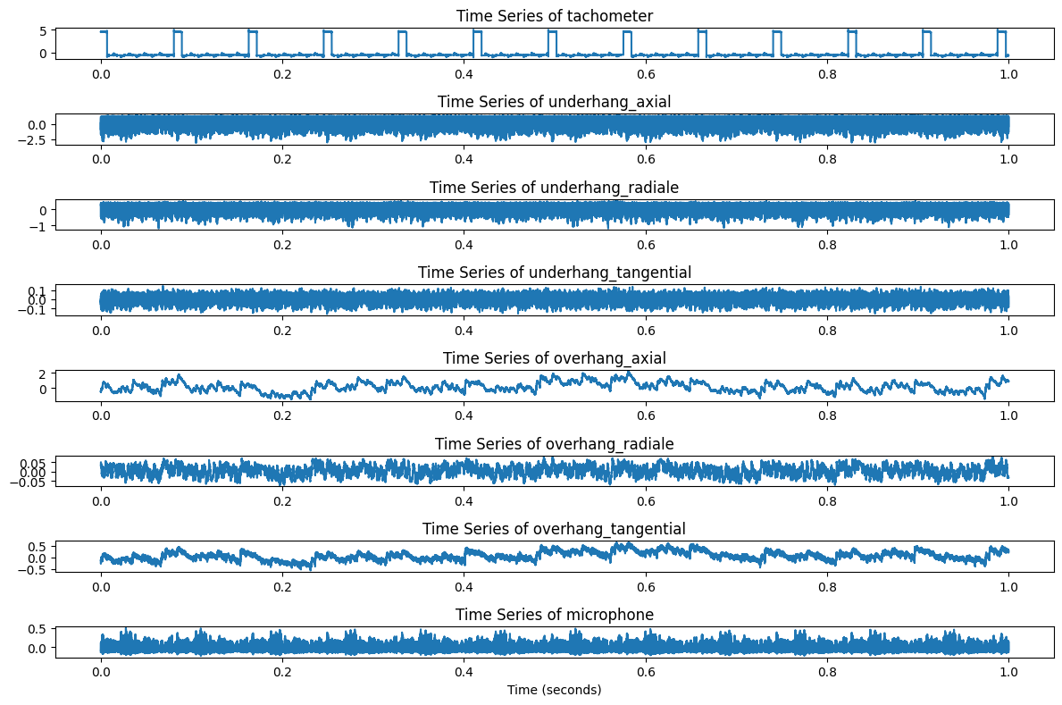
2. Feature Engineering
High-frequency time-series data can be noisy and large, so feature engineering becomes crucial. Two primary transformations were used in FeatureEngineering.ipynb and ultimately in the main pipeline:
- Downsampling: Consolidates raw data by averaging every b samples. In the repository,
b=2500was used, reducing 250,000 samples per file to just 100 samples.
- Rolling Mean: Applies a moving average (with a given window size) to smooth abrupt fluctuations and incorporate temporal context into each feature.
In FeatureEngineering.ipynb, you’ll see:
def downSampler(data, b):
"""
Downsamples the given DataFrame by averaging every 'b' rows.
"""
return data.groupby(data.index // b).mean().reset_index(drop=True)
def rolling_mean_data(df, window_size=100, columns=None):
"""
Applies a rolling mean transformation to specified columns.
"""
if columns is None:
columns = df.select_dtypes(include=[np.number]).columns
df_copy = df.copy()
df_copy[columns] = df_copy[columns].rolling(window=window_size, min_periods=1).mean()
return df_copy
# Usage:
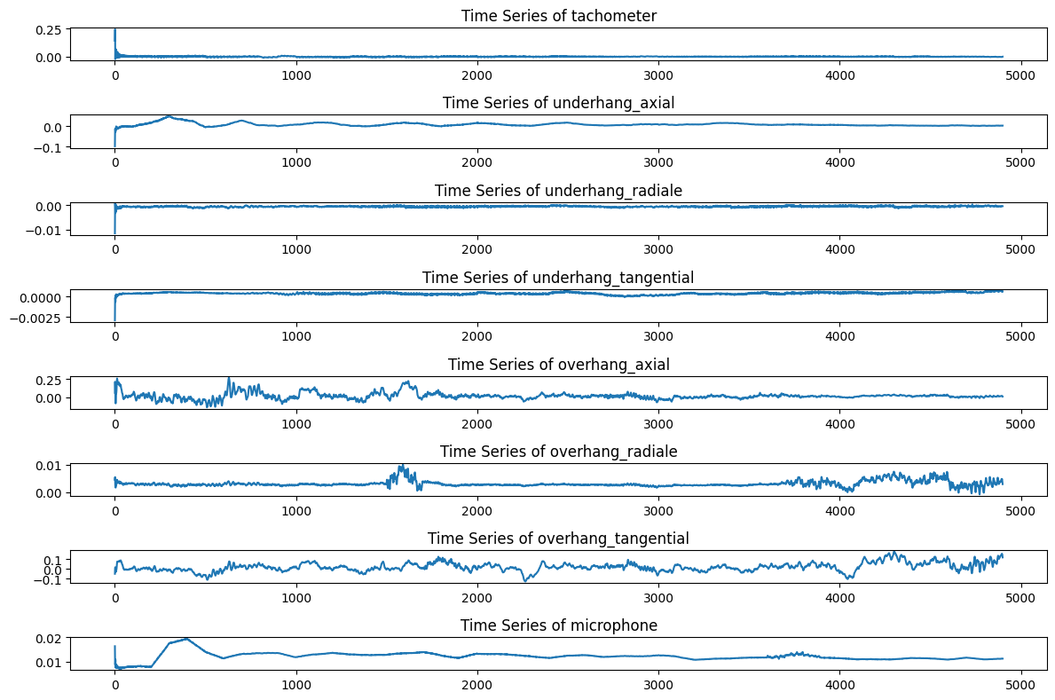
normal_df = downSampler(normal_df, 2500)
normal_df = rolling_mean_data(normal_df, window_size=100)After applying both transformation, the behaviour of each feature across the time is presented below:
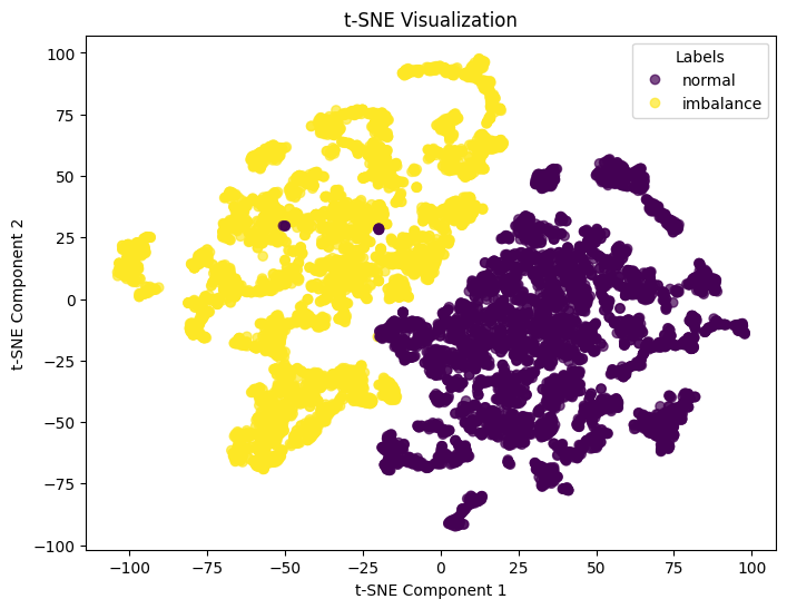
t-SNE Visualization for Feature Separability
After feature transformations, we often test whether the classes (normal vs. imbalance) are more distinguishable, and we can visually check this using dimensionality reduction methods such as Principal component analysis for linear transformation or t-distributed Stochastic Neighbor Embedding for non-linear transformation. In this case, we apply t-SNE as it is capable of dealing with non-linear transformation.
from sklearn.manifold import TSNE
from sklearn.preprocessing import StandardScaler

def plot_tsne(df, label_column='label'):
    features = df.select_dtypes(include=[np.number]).drop(columns=[label_column], errors='ignore')
    features_scaled = StandardScaler().fit_transform(features)

    tsne = TSNE(n_components=2, perplexity=30, random_state=42)
    tsne_results = tsne.fit_transform(features_scaled)

    # Plot
    plt.figure(figsize=(8, 6))
    plt.scatter(tsne_results[:, 0], tsne_results[:, 1], c=df[label_column], cmap="viridis", alpha=0.7)
    plt.title("t-SNE Visualization")
    plt.show()
The following t-SNE plot clearly shows how both classes can be distinguished visually. This visualization gives us confidence that there is a non-linear transformation capable of producing a rule that will correctly classify the binary time-series dataset.
3. Building & Training a Multi-Layer Perceptron (MLP) in PyTorch
While more sophisticated sequence models (e.g., LSTM, 1D CNNs) are more relevant for time-series data, a Multi-Layer Perceptron is a basic architecture that does not intrinsically include temporal dependencies. Since we have applied feature engineering capable of introducing basic temporal effects to features, the MLP might be sufficient for correctly classify this dataset. In general, if sequential dependencies matter, alternatives like RNN, LSTM, 1-D CNN, or Transformers may perform better, whereas MLP is effective for feature-based classification when raw time series is converted into useful representations through feature engineering.
3.1 The Dataset & DataLoader
In PyTorch, we create a custom Dataset class to handle how features and labels are fed to the model:
import torch
from torch.utils.data import Dataset, DataLoader

class MachineryDataset(Dataset):
    def __init__(self, data, label_column='label'):
        self.labels = data[label_column].values.astype(np.float32)
        self.features = data.drop(columns=[label_column, 'time'], errors='ignore').values.astype(np.float32)

    def __len__(self):
        return len(self.features)

    def __getitem__(self, idx):
        x = self.features[idx]
        y = self.labels[idx]
return x, y__getitem__: Returns a single sample(features, label).__len__: Provides the total length of the dataset.
We also build a DataLoader object that batches the data and shuffles it during training:
train_dataset = MachineryDataset(all_data, label_column='label')
train_loader = DataLoader(train_dataset, batch_size=64, shuffle=True)
3.2 MLP Model Architecture
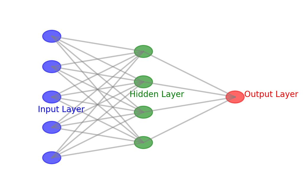
A simple feed-forward neural network can be built using fully connected layers (nn.Linear):
import torch.nn as nn

class TimeSeriesMLP(nn.Module):
    def __init__(self, input_dim, hidden_dim, n_layers, dropout_prob=0.3):
        super(TimeSeriesMLP, self).__init__()
        layers = []
        layers.append(nn.Linear(input_dim, hidden_dim))
        layers.append(nn.ReLU())
        layers.append(nn.Dropout(dropout_prob))

        for _ in range(n_layers - 1):
            layers.append(nn.Linear(hidden_dim, hidden_dim))
            layers.append(nn.ReLU())
            layers.append(nn.Dropout(dropout_prob))

        layers.append(nn.Linear(hidden_dim, 1))
        layers.append(nn.Sigmoid())

        self.net = nn.Sequential(*layers)

    def forward(self, x):
        return self.net(x)
Hidden Layers and Activation:
The model consists of
n_layershidden layers, each applying a linear transformation (nn.Linear), followed by ReLU activation (nn.ReLU()).ReLU (Rectified Linear Unit) is used because it helps mitigate the vanishing gradient problem and accelerates training.
Dropout Regularization:
A dropout layer (
nn.Dropout(dropout_prob)) is applied after each hidden layer to reduce overfitting.Dropout randomly disables a fraction of neurons during training, forcing the model to learn more robust features.
Output Layer and Activation:
The final layer maps the last hidden representation to a single output neuron using
nn.Linear(hidden_dim, 1).Sigmoid activation (
nn.Sigmoid()) is applied to ensure the output is in the range [0, 1], making it suitable for binary classification.
3.3 Training Loop
The train_model function in src/main.py file trains the MLP using a binary classification approach, tracking both loss and accuracy.
import torch.optim as optim
import torch

def train_model(model, train_loader, val_loader, epochs=50, lr=0.0005):
    criterion = nn.BCELoss()
    optimizer = optim.Adam(model.parameters(), lr=lr)

    history = {
        'train_loss': [], 'val_loss': [], 'train_acc': [], 'val_acc': []
    }

    for epoch in range(epochs):
        model.train()  # Enable training mode
        epoch_train_loss = 0
        correct_train = 0
        total_train = 0

        for inputs, targets in train_loader:
            optimizer.zero_grad()
            outputs = model(inputs).squeeze()  # Forward pass
            loss = criterion(outputs, targets)  # Compute loss
            loss.backward()  # Backpropagation
            optimizer.step()  # Update weights

            epoch_train_loss += loss.item()
            preds = (outputs > 0.5).float()  # Convert probabilities to binary predictions
            correct_train += (preds == targets).sum().item()
            total_train += targets.size(0)

        train_accuracy = correct_train / total_train  # Compute training accuracy

        model.eval()  # Enable evaluation mode
        epoch_val_loss = 0
        correct_val = 0
        total_val = 0

        with torch.no_grad():
            for inputs, targets in val_loader:
                outputs = model(inputs).squeeze()
                val_loss = criterion(outputs, targets)
                epoch_val_loss += val_loss.item()

                preds = (outputs > 0.5).float()
                correct_val += (preds == targets).sum().item()
                total_val += targets.size(0)

        val_accuracy = correct_val / total_val  # Compute validation accuracy

        # Store metrics for analysis
        history['train_loss'].append(epoch_train_loss / len(train_loader))
        history['val_loss'].append(epoch_val_loss / len(val_loader))
        history['train_acc'].append(train_accuracy)
        history['val_acc'].append(val_accuracy)

        print(f"Epoch {epoch+1}/{epochs}, Validation Loss: {epoch_val_loss / len(val_loader):.4f}, Validation Accuracy: {val_accuracy:.4f}")

return history- Binary Cross-Entropy Loss (
nn.BCELoss()):- Suitable for binary classification, where the target labels are
0or1.
- Suitable for binary classification, where the target labels are
- Adam Optimizer (
optim.Adam()):- Adaptive learning rate for better convergence.
- Accuracy Tracking:
- Uses thresholding (
outputs > 0.5) to determine class predictions. - Compares predictions to true labels (
targets) to compute accuracy.
- Uses thresholding (
- Training & Validation Loss History:
- Logs loss and accuracy at each epoch for performance monitoring.
4. Putting It All Together
Finally, in src/main.py we orchestrate the entire workflow: 1. Data Ingestion & Labeling
2. Feature Engineering (Downsampling, Rolling Mean, StandardScaler)
3. Splitting (Time-series split into train/val/test sets)
4. MLP Training
5. Evaluation: Accuracy, F1, Precision, Recall, AUC-ROC
Below is a condensed snippet showing the pipeline’s main logic:
# Load normal and imbalance data
normal_dfs = load_filtered_dfs(data_path, "normal")
imbalance_dfs = load_filtered_dfs(data_path, "imbalance-6g")

# Apply augmentation (downsampling + rolling) to each DF, then concat
normal_df = pd.concat([augment_features(df) for df in normal_dfs], ignore_index=True)
imbalance_df = pd.concat([augment_features(df) for df in imbalance_dfs], ignore_index=True)

# Label the data
normal_df["label"] = 0
imbalance_df["label"] = 1

all_data = pd.concat([normal_df, imbalance_df], ignore_index=True)

# Show correlation matrix
save_correlation_matrix(all_data)

# t-SNE visualization
plot_tsne(all_data, label_column='label', output_file="../figures/tsne_visualization.png")

# Time-series split (train/val/test)
train_data, val_data, test_data = time_series_split(all_data)

# Normalize features
scaler = StandardScaler()
train_data.iloc[:, :-1] = scaler.fit_transform(train_data.iloc[:, :-1])
val_data.iloc[:, :-1] = scaler.transform(val_data.iloc[:, :-1])
test_data.iloc[:, :-1] = scaler.transform(test_data.iloc[:, :-1])

# Datasets & Loaders
train_dataset = MachineryDataset(train_data)
val_dataset = MachineryDataset(val_data)
test_dataset = MachineryDataset(test_data)

train_loader = DataLoader(train_dataset, batch_size=32, shuffle=False)
val_loader = DataLoader(val_dataset, batch_size=32, shuffle=False)

# Initialize and train MLP
model = TimeSeriesMLP(
    input_dim=train_dataset.features.shape[1],
    hidden_dim=3,
    n_layers=2
)
history = train_model(model, train_loader, val_loader)  # default epochs=50

# Evaluate
test_loader = DataLoader(test_dataset, batch_size=32, shuffle=False)
test_metrics = evaluate_model(model, test_loader)
plot_evaluation_results(test_metrics, output_file="../figures/evaluation_plot.png")
Evaluation & Metrics
After training, we apply the model to the test set. For binary classification, we typically measure:
- Accuracy: Ratio of correct predictions over total.
- F1-score: Harmonic mean of precision & recall.
- Precision: Among predicted positives, how many are truly positive?
- Recall: Among all actual positives, how many did we predict correctly?
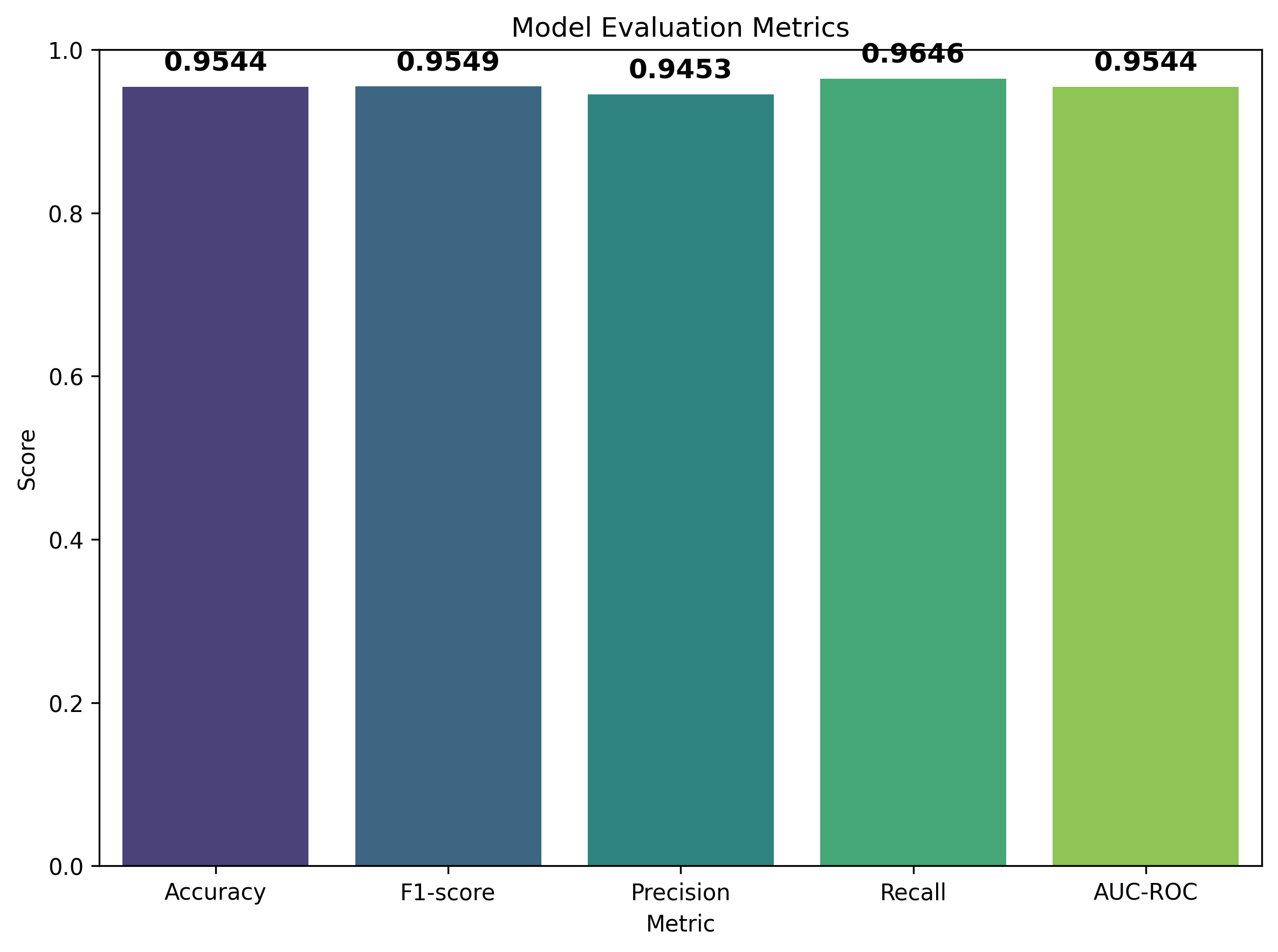
Excellent performance, which suggests that even a relatively straightforward MLP can separate normal vs. imbalance classes well, thanks to feature engineering (downsampling + rolling mean).
5. Next Steps & Enhancements
- Hyperparameter Optimization
- Test different hidden layer sizes, dropout probabilities, and learning rates.
- Consider
GridSearchorBayesian Optimizationfor an automated approach.
- Test different hidden layer sizes, dropout probabilities, and learning rates.
- Include More Fault Conditions
- The MAFAULDA dataset has multiple fault types (unbalance, misalignment, bearing faults). Extending beyond just normal vs. imbalance classification can add realism.
- Sequence Models
- For a deeper time-series approach, experiment with CNNs (1D Convolutions) or LSTM architectures. Those are better at capturing sequential dependencies without relying only on rolling averages.
- Real-Time Inference
- Deploy the trained model in a streaming or edge environment for real-time fault detection in industrial settings.
Conclusion
We’ve walked through the basic steps to a complete pipeline for classifying mechanical faults using time-series data. The key lessons include:
- EDA is indispensable for quickly assessing data quality and distributions.
- Feature Engineering (downsampling, rolling means) can convert raw time series into useful representations to train deep learning models that does not include temporal dependencies inherently.
- Even a basic MLP can achieve high accuracy if the features reflect the underlying process well.
- Evaluation metrics (Accuracy, F1, Precision, Recall) are critical to understand true performance.
If you’re looking to adapt this pipeline to your own fault classification tasks—whether it’s rotating machinery, bearings, or other mechanical equipment—these concepts should be straightforward to customize. Feel free to explore the MAFAULDA dataset for your own experiments or extend it with advanced deep learning architectures.
Thanks for reading, and happy fault detecting!